
Delays between ECG fiducials, PPG upstrokes or peaks, and mechanical J landmarks. Retain both the typical delay and its variation.
Data & features
Timing, magnitude, shape—and their variability
Inspect timing, magnitude and shape measurements from ECG, PPG and bed-based BCG. These descriptive views explain the model inputs; held-out predictions and the calibration protocol are on the prediction-results page.
Participants and recordings
The Carlson dataset supplies synchronized recordings from 40 participants. This report uses the first 100 detected heartbeats after five seconds of each recording, with ECG, finger PPG, Film0 and LC_BCG0 bed sensors. Analysis uses processed signals sampled at 1 kHz; display traces are reduced to 100 Hz.
Two sets of BCG sensors: four electromechanical films beneath the mattress (Film0–Film3), and four load cells beneath the corner bedposts (LC_BCG0–LC_BCG3). Both sets record tiny heartbeat-related mechanical movements, called ballistocardiography (BCG); they differ in sensing technology and location. This analysis uses Film0 and LC_BCG0, alongside ECG and finger PPG. The four-feature reproduction uses Film0 alone. Film0 is the film sensor nearest the head end of the bed; the “0” identifies a sensor, not a processing stage. LC_BCG0 is the BCG channel from load cell 0. Carlson et al., Section 2.1 and Figure 2 describe the arrangement.
Reference systolic and diastolic pressure are the maximum and minimum of Finometer-reconstructed brachial pressure in each ECG cycle. Prediction evaluation includes all 40 participants and 1,030 valid five-beat windows (16–26 per person). Missing landmarks remain missing rather than joining nonadjacent beats. Reference and quality rules.
Select a participant below to inspect their signals and descriptors. The descriptive explorer includes all 46 extracted candidates; prediction retains 42 after a calibration-only redundancy screen. Feature selection.
Separate acquisition-scale magnitude from unit-range shape: amplitude, rise time, width, slopes and profile differences.
Summarize feature distributions and successive changes; compare ensembles with different alignments to inspect timing jitter.
Timing between signals
One inspected cycle, with the surrounding signal for context. Each row has its own voltage scale.
Vertical colored markers show automatically detected events. Dashed gray lines bound the ECG cycle. PPG “rise” means maximum positive slope, not the pulse foot. Display traces are antialias-resampled to 100 Hz; numerical timings use the original 1 kHz indices.
Timing variability
Delays remain attached to their original cycles, including gaps for missing landmarks.
SD and variance describe spread across beats; RMSSD describes changes between adjacent valid beats. Missing beats are never bridged. These are descriptive measurements of variability in this excerpt, not estimates of uncertainty in the detector.
Magnitude versus shape
Left: acquisition-scale voltage with peak-to-trough span. Right: subtract the cycle minimum and divide by its span, producing a unit-range profile. Rise time uses 10–90% of the leading trough-to-peak excursion; width uses the contiguous half-height crossings around the maximum. Missing crossings remain unavailable. Beat curves retain every tenth sample and original extrema for display; measurements use every original sample. These generic pulse descriptors do not define clinical ECG intervals.
Variation across waveforms
Median profiles with empirical 10–90% bands across the participant's eligible cycles.
A broad phase-aligned band can reflect timing shifts, shape changes or both. Own-landmark alignment helps inspect this distinction; it is not a formal decomposition. Shape residual is RMS distance from this person's median normalized profile on supported phase samples. The template is descriptive and must be learned within training data if later used for prediction.
Features and reference blood pressure
Contrast differences between people with beat-to-beat relationships within one person. No predictive model is fitted.
Left: each dot is one participant; feature and BP summaries use their own valid cycles, with at least 50 required for each. Click a person to inspect their beats on the right. Right: paired, unsmoothed measurements from the same ECG cycle, colored by recording time. Changing the feature summary affects only the left plot.
Each dot is one participant's within-person correlation (at least 10 paired valid cycles). The range can reveal different or opposing relationships that a pooled beat scatterplot would conceal. Constant series have no defined correlation. Valid counts differ by feature.
Compare all extracted features
Fixed feature-family order, without ranking by the strongest correlation. Select a feature to inspect its scatterplots.
| Feature | Across people | People | Median within-person correlation | Within-person range | People |
|---|
These are exploratory, same-excerpt associations, not evidence of predictive accuracy or causation. Adjacent beats are autocorrelated; no independent-beat p-values or significance stars are shown. Shared time trends, heart rate, sensor coupling and fiducial errors can contribute to correlations. Participant averages can reflect between-person differences without tracking pressure within a person. Full-cohort screening must not be used to select features before an evaluation split.
How the measurements are organized
Processed input signalsECG · PPG · film / load-cell BCG
→Cycle & landmark tableParticipant, beat ID, time, QC flags
→Beat-level descriptorsTiming · magnitude · shape
→Model-ready summariesTypical value · variability · valid count
| Family | Candidate measurements | Across-beat summary | Status |
|---|---|---|---|
| Original BCG features | log I–J duration, log J–K duration, I–J amplitude, J–K amplitude | Trailing five-beat means for both predictive approaches | Retained in the 42-feature model and the four-feature comparison. |
| Inter-waveform timing | ECG → PPG rise / peak, ECG → Film J, Film J → PPG rise, Film J → load-cell J; I–J / J–K intervals in both BCG channels; RR duration | Median, SD, variance, IQR, 10–90% range; adjacent-beat RMSSD | Beat-level timings enter the personalized waveform model. |
| Magnitude | Peak-to-trough voltage, median offset, median-centered RMS, maximum upstroke slope | Distribution of the scalar features; median-centered voltage ensemble | Extracted candidate descriptors. Voltage reflects acquisition gain and sensor contact. |
| Shape | Unit-range profiles; rise time, half-height width; RMS profile residual | Median profile, pointwise 10–90% bands, distribution of residuals | Beat-level shape descriptors enter the personalized waveform model; shape-residual templates use training data only. |
Each descriptor stays aligned to a participant, detected beat and original sample time. Prediction uses trailing five-beat means, with imputation and scaling learned from calibration data. Variability bands and correlations here describe the observed excerpt and are not additional regression inputs.
BCG landmarks and the source features
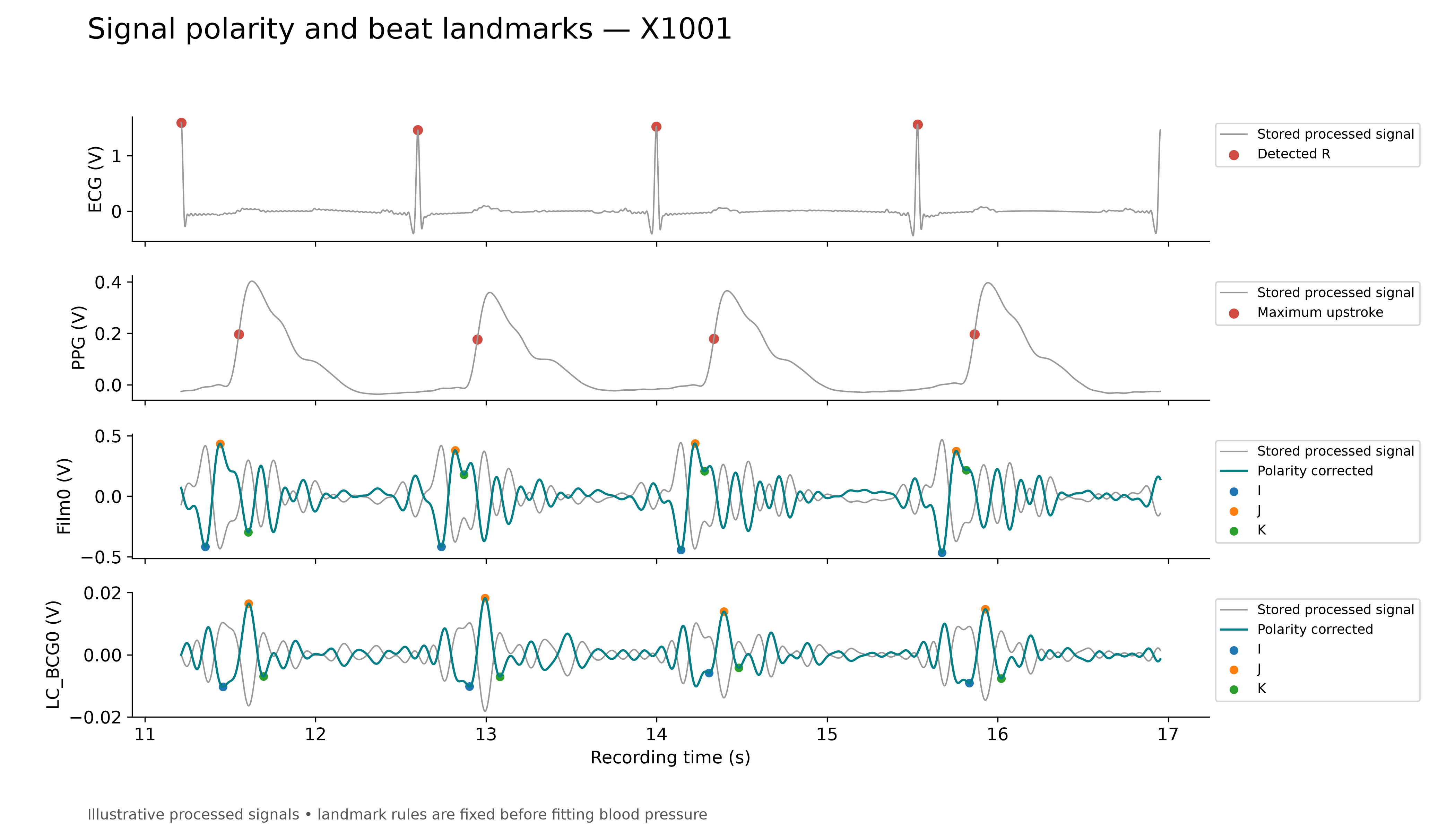
J is a prominent mechanical peak after the ECG fiducial; I and K are neighboring minima. The original four predictors describe the I–J and J–K durations and amplitude differences. Source method.
Alignment and interpretation
Compare cycle-aligned profiles with profiles centered on each waveform's own landmark. Shaded bands show variation across observed beats, not confidence intervals. Normalizing shape removes overall gain and offset, but does not remove motion, timing differences or detector errors. Alignment and variability explain how to read these views.
The descriptive profiles summarize the observed excerpt. Predictive models learn their waveform templates within calibration data only; their accuracy is evaluated separately on the results page. Feature definitions describe the measurements and the 42-feature selection.
Ensemble figure (PDF) · Timing variability (PDF) · Build provenance · Dataset · Original study