Spatial resemblance and concentration measure different things AI

Why a strong spatial correlation need not mean that most of a pattern lies inside a reference system.

When naming a learned pattern after a reference system, two questions easily become conflated: does its spatial profile resemble that system, and how much of its weight lies there? Correlation answers the first; concentration answers the second. Neither alone establishes a functional identity.

Resemblance depends on spatial contrast

Suppose $s_i$ is a nonnegative regional weight and $m_i$ indicates membership in a reference system. Pearson correlation compares their centered profiles,

$$r=\frac{\sum_i(s_i-\bar s)(m_i-\bar m)}{\sqrt{\sum_i(s_i-\bar s)^2\sum_i(m_i-\bar m)^2}}.$$

Multiplying every $s_i$ by a positive constant leaves $r$ unchanged. Adding a constant also leaves it unchanged: correlation measures relative spatial contrast after centering, rather than absolute amount. The SciPy definition of Pearson correlation gives the corresponding formula and undefined constant-input case.

Two profiles differing only by a uniform background have identical Pearson correlation but different fractions of weight in the reference.

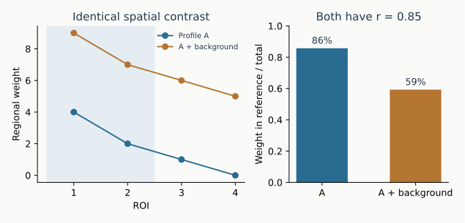
Illustrative four-ROI profiles. The reference contains the first two ROIs. Adding background weight preserves similarity but reduces concentration from 86% to 59%.

Concentration depends on the denominator

A weight share is $q=\sum_i m_i s_i/\sum_i s_i$. It changes when background weight increases, but remains unchanged when the whole pattern is uniformly rescaled. Thus neither correlation nor share measures total contribution to the recorded signal. That requires the pattern’s scale together with its time-dependent expression, evaluated in a consistent model convention.

For signed networks, summarize positive and negative magnitudes separately before calculating either quantity. This avoids cancellation between poles. When regional weights are off-diagonal edge sums, the share allocates edge endpoints: an edge connecting two different systems contributes to both regional footprints. It is not the fraction of edges entirely within a system.

Reference size and spatial dependence also matter. A large system can receive substantial weight without selective localization, and neighboring parcels are not independent observations. Correlation and share are descriptive evidence; statistical localization requires a suitable spatial null and a specified comparison question. The Schaefer atlas documentation explains how parcel names relate to the reference networks used here.